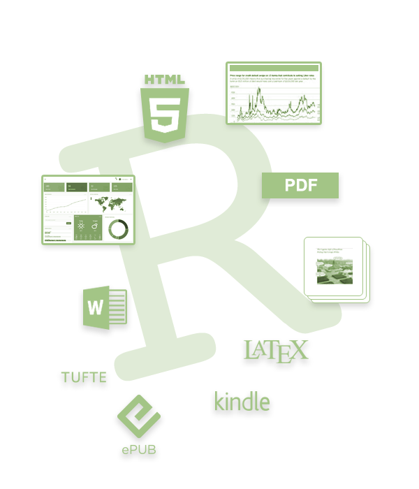
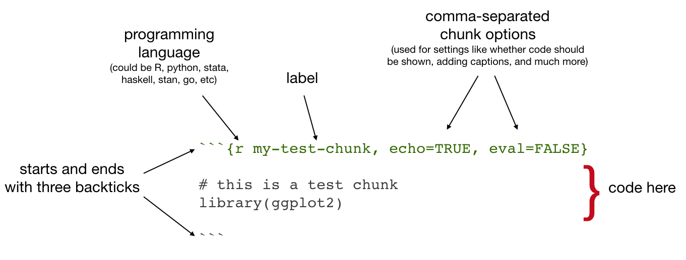
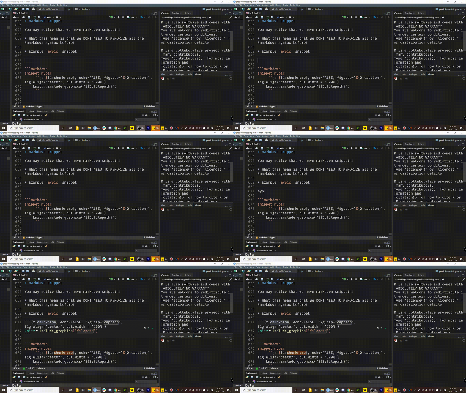
class: center, middle, inverse, title-slide # Lecture 1 ## Github, Kaggle, and R Markdown ### Issac Lee ### 2021-02-25 --- class: center, middle # Sungkyunkwan University  ## Actuarial Science --- class: center, middle # Predictive modeling with R --- class: inverse, center, middle # Instructor --- # Issac Lee  * The University Of Iowa, Statistics & Actuarial Science * SungKyunKwan University, Actuarial Science * Website: [theissaclee.com](https://www.theissaclee.com/) --- # Research Interests * Pay-How-You-Drive insurance telematics data * Replacing nested monte carlo simulation in insurance product valuation process * Machine learning in Actuarial Science * Graph theory & Spatial Statistics --- class: inverse, center, middle <img src="./hammer.svg" width="15%" style="display: block; margin: auto;" /><img src="./ice-cube.svg" width="15%" style="display: block; margin: auto;" /> # Tell me about you --- class: inverse, center, middle # Lecture Intro. --- .pull-left[ # Basic Info. * Friday 9 am. - 12 am. * Zoom will be provided * Two 10 min. breaks ] .pull-right[ # Our goal * Find your **RESEARCH TOPIC** * Explore many ML methodology * Solid background about **Models** * Solid background about **R** * Modeling and Visualization * Documentation * How to collaborate with other people (Team codebook) ] --- # Course Info. * E-mail: sak-lee@uiowa.edu * Please use **[SKKU:5155]** in your email subject * Textbook - An Intro. to Statistical Learning * Reference: - Applied Predictive modeling - Feature Engineering and selection --- # Course Topics ### Setup * Github, Kaggle, R markdown ### R programming * `tidyverse`, `tidymodels`, `torch` ### Statistical Models * Regression, Classification, Tree-Based method, Deep-learning --- # Course Activities - Identify 3 candidate papers of different topics from the paper list. One will be assigned for presentation. * Literature Review - Submit a 1500-words summary of the assigned paper * Paper presentation - Present the paper in one of the classes. (20 min.) - Prepare questions to ask the presenters you are assigned to review, and submit your comments --- # Course Activities 2 * Form groups of three and sign up your group by next week * Homework - 20% * Indivisual Presentation - 30% * Literature review (LR) – 20% - Propose topic and provide a list of at least 5 papers, more preferred. - Submit final LR document * Course project (CP) (30%) * Proposal document & mid-term presentation, final presentation & report --- # Course Activities 3 * **Apply** methods learned in the course to solve an important problem. * **Evaluate and compare** the performance of state-of-the-art methods on a problem * Methodological innovation is not required, but encouraged. Each group **MUST** have at least one meeting with me during office hours to discuss LR & CP topic. --- class: inverse, middle, center <img src="./question.svg" width="30%" style="display: block; margin: auto;" /> # Questions? .footnote[Icons made by Freepik from flaticon.com] --- <iframe width="1300" height="600" src="https://www.youtube.com/embed/s3JldKoA0zw?version=3&rel=0" frameborder="0" allow="accelerometer; encrypted-media; gyroscope; picture-in-picture" allowfullscreen></iframe> --- # Set up **RStudio** Cloud * Sign up for a free RStudio Cloud account at https://rstudio.cloud/ * Recommend logging in with an existing Google or GitHub account * I want you to be able to work from your own laptop in this workshop, but Cloud is **an important back-up plan** should you run into troubles. --- # R markdown .pull-left[ * R + Markdown * We know R part * How about Markdown part? * [Markdown 10-minute interactive tutorial](https://commonmark.org/help/tutorial/) Pandoc takes care of markdown part. Pandoc is a universal document converter, which is written in [Haskell](https://www.haskell.org/). ] .pull-right[  ] --- # The Knitting process When we knitr the Rmd document, R generates md file, and it will be passed to pandoc!  * Possible outcomes: PDF(LaTex), HTML, Word file, epub file.. * [Gallery](https://rmarkdown.rstudio.com/gallery.html) --- # Anatomy of an Rmd file ````markdown --- title: "Here is the title" date: 2021-02-23 output: html_document --- ```{r setup, include=FALSE} library(tidyverse) ``` # Normal Distribution Actually, Normal distribution is not normal, it's so special in Stat. ```{r} x <- rnorm(100) y <- rnorm(100) plot(x, y) ``` ```` --- # YAML header ("YAML Ain't Markup Language") ````markdown *--- *title: "Here is the title" *date: 2021-02-23 *output: html_document *--- ```{r setup, include=FALSE} library(tidyverse) ``` # Normal Distribution Actually, Normal distribution is not normal, it's so special in Stat. ```{r} x <- rnorm(100) y <- rnorm(100) plot(x, y) ``` ```` --- # Body (Plain Text part) ````markdown --- title: "Here is the title" date: 2021-02-23 output: html_document --- ```{r setup, include=FALSE} library(tidyverse) ``` *# Normal Distribution * *Actually, Normal distribution is not normal, it's so special in Stat. ```{r} x <- rnorm(100) y <- rnorm(100) plot(x, y) ``` ```` --- # Code ("Not only R code") ````markdown --- title: "Here is the title" date: 2021-02-23 output: html_document --- *```{r setup, include=FALSE} *library(tidyverse) *``` # Normal Distribution Actually, Normal distribution is not normal, it's so special in Stat. *```{r} *x <- rnorm(100) *y <- rnorm(100) *plot(x, y) *``` ```` --- class: inverse, middle, center # Basic Syntax --- class: syntax-slide .pull-left[ ### This... \*italics\* and \*\*bold\*\* <span>`</span> inline code` sub~2~/superscript^2^ \~\~strikethrough\~\~ escaped: \\* \\_ \\\ endash: --, emdash: --- \> blockquote \# Header 1 ] .pull-right[ ### turns into this... *italics* and **bold** `inline code` sub<sub>2</sub>/superscript<sup>2</sup> ~~strikethrough~~ escaped: \* \_ \\ endash: –, emdash: — > blockquote # Header 1 ] --- class: syntax-slide .pull-left[ ### This... \- unordered list <br> \- sub-item <br> \- sub-sub-item 1\. ordered list <br> 1\. item 2 <br> \- sub-item 1 <br> inline-math: $A = \pi*r^{2}$ math-block: <span>$</span>$A = \pi*r^{2}$$ ] .pull-right[ ### turns into this... - unordered list - sub-item - sub-sub-item 1. ordered list 1. item 2 <br> i. sub-item 1 <br> inline-math: `\(A = \pi*r^{2}\)` math-block: `$$A = \pi*r^{2}$$` ] --- class: inverse, middle, center <img src="./code.svg" width="30%" style="display: block; margin: auto;" /> # Code .footnote[Icons made by Freepik from flaticon.com] --- class: small-font # Code chunks  --- # Some chunk options - `echo`: whether or not to display code in knitted output - `eval`: whether or to to run the code in the chunk when knitting - `include`: whether to include anything from the from a code chunk in the output document --- # Setup chunk ````markdown ```{r setup, include=FALSE} # don't show code unless we explicitly set echo = TRUE knitr::opts_chunk$set(echo = FALSE) ``` ```` - Normally, an R Markdown document starts with a chunk that's used to set some options and load required libraries. - `knitr::opts_chunk$set` sets default options for all chunks. --- # Including images .pull-left[ ````markdown ```{r chunkname, fig.cap="picture caption", fig.align="center", out.width="50%"} knitr::include_graphics("markdown.png") ``` ```` ] .pull-right[ <div class="figure" style="text-align: center"> <img src="./question.svg" alt="picture caption" width="50%" /> <p class="caption">picture caption</p> </div> ] --- # Inserting plot .pull-left[ ````markdown ```{r} cars %>% ggplot() + aes(x = speed, y = dist) + geom_point() ``` ```` ] .pull-right[ ```r cars %>% ggplot() + aes(x = speed, y = dist) + geom_point() ``` <img src="lec1_files/figure-html/unnamed-chunk-2-1.png" width="60%" style="display: block; margin: auto;" /> ] --- # Tables .pull-left[ ````markdown ```{r} knitr::kable(head(as.tibble(mtcars[,1:3]), 5), position = "!h", col.names = c("col1", "col2", "col3"), caption = "caption", align = "lrc", booktab = TRUE) ``` ```` ] .pull-right[ ``` ## Warning: `as.tibble()` is deprecated as of tibble 2.0.0. ## Please use `as_tibble()` instead. ## The signature and semantics have changed, see `?as_tibble`. ## This warning is displayed once every 8 hours. ## Call `lifecycle::last_warnings()` to see where this warning was generated. ``` Table: caption |col1 | col2| col3 | |:----|----:|:----:| |21.0 | 6| 160 | |21.0 | 6| 160 | |22.8 | 4| 108 | |21.4 | 6| 258 | |18.7 | 8| 360 | ] --- # Inline code Inside your text you can include code with the syntax <span>`</span> r code here` . For example, <span>`</span> r 4 + 4` would output 8 in your text. ```r dim(diamonds) ``` ``` ## [1] 53940 10 ``` ```r num_diamonds <- nrow(diamonds) ``` .pull-left[ There are <span>`</span> r num_diamonds` rows in the `diamonds` dataset. ] .pull-right[ There are 53940 rows in the `diamonds` dataset. ] --- class: larger-body # Inline code with python At the moment, syntax like <span>`</span> python code here` is not valid. However, you can use the [`reticulate`](https://rstudio.github.io/reticulate/articles/r_markdown.html) package to access variables from python chunks. ````markdown ```{python} my_number = 4 + 8 ``` ```` ````markdown ```{r} library(reticulate) py$my_number ``` ```` ```r py$my_number ``` ``` ## [1] 12 ``` `my_number` can be referred inline by <span>`</span> r py$my_number` . --- class: center, middle, inverse # Useful tips --- # Very Important `Alt` + `Shift` + `K` shows all shortcuts! However, some are USEFUL, some are **NOT**! ### Useful **Shortcuts!** .pull-left[ add `%>%` operator: `Ctrl` + `Shift` + `m` add `<-` operator: `Alt` + - add cursors! : `Ctrl` + `Alt` + down or up search functions: `Ctrl` + . search commands: `Ctrl` + `Shift` + `p` ] .pull-right[ Run current chunk: `Ctrl` + `Alt` + `c` R code re-formatting: `Ctrl` + `Shift` + `a` Copy current below: `Shift` + `Alt` + down Insert `R` code chunk: `Ctrl` + `Alt` + i ] --- # Very Very Important Modify and Make your own shortcuts! `Tools` > `Modify Keyboard Shortcuts` will open another door to you. For example, * Insert `python` code: `Ctrl` + `Alt` + p * Insert snippet: `Shift` + `Space` --- # `\(Very^\infty\)` Important **Snippet** save your time, almost 1 year during your whole life, no joke. .pull-left[ ### What the hack is snippet * **Text macros** that are used for quickly inserting common snippets of code * `Tools` > `Global option` > `Code` > `Snippet` * Some people know there are *code snippet* in Rstudio ] .pull-right[ <div class="figure" style="text-align: center"> <img src="./snippet.jpg" alt="Available snippets languages" width="80%" /> <p class="caption">Available snippets languages</p> </div> ] --- # Markdown snippet You may notice that we have markdown snippet!! * You **DONT NEED TO MEMORIZE** all the Rmarkdown syntax! .pull-left[ * Example `mypic` snippet ````markdown snippet mypic ```{r ${1:chunkname}, echo=FALSE, fig.cap="${2:caption}", fig.align='center', out.width = '100%'} knitr::include_graphics("${3:filepath}") ``` ```` ] .pull-right[  ] --- # Snippet is in action --- # **R**Markdown packages .pull-left[ * **Pagedown**: single html document generation * **Bookdown** - pdf, epub, or html book * Writing a gitbook like [Prof. Tierney](http://homepage.stat.uiowa.edu/~luke/classes/STAT7400-2021/_book/index.html) * **Blogdown** - Static website builder Hugo wrapper * Personal website like [me](theissaclee.com) * Theme: Academy, Apero (is developing by Rstudio) ] .pull-right[ * **Distill**: if you really like minimalizm. * Concept is developed by Google, package developed by Rstudio. * Suitible for academic writing * **Xaringan**: Presentation * Like the one you're looking at. * `xaringan themer` - Easy theming package * **Thesisdown**: Thesis with Rmd. ] --- # Set up GitHub * Using GitHub in this lecture for **version control** and **publishing**. * Sign up for a GitHub.com account at https://github.com/join * Complete these installation instructions. * Test your connection between GitHub and RStudio following these steps. * you choose HTTPS over SSH, and * you setup a GitHub Personal Access Token. --- # Check out your default branch * `main` as the default branch for all new repositories * To check this, for user accounts, go to: https://github.com/settings/repositories * You should see something like this: <img src="./mainbranch.jpg" width="50%" style="display: block; margin: auto;" /> If yours still says master, you may change it to main here if you wish. --- # Github Intergration ```r install.packages(c("usethis", "remotes")) remotes::install_github("rstudio/rmarkdown") ``` ```r rmarkdown::pandoc_version() ``` ``` ## [1] '2.11.4' ``` ### Set up your Github PAT(Personal Access Token) To use `usethis` package, you need to set up PAT. Instruction is here: https://happygitwithr.com/credential-caching.html#get-a-pat --- # Publish your self in online ```r install.packages("postcards") ``` * Restart your R session. * If you use RStudio, use the menu item Session > Restart R * Ctrl + Shift + F10 (Windows and Linux) or * Command + Shift + F10 (Mac OS). ```r packageVersion("postcards") ``` ``` ## [1] '0.2.0' ``` --- # Create GitHub repo We’ll follow a “New Project, GitHub first” workflow. * Go online to your GitHub account * Create a new repository and YES initialize this repository by adding a README file. ```r usethis::create_from_github("username/my-postcard", destdir = "/pathto/project") ``` in RStudio Cloud see this link: https://bren.zendesk.com/hc/en-us/articles/360015826731-How-to-connect-RStudio-Cloud-with-Github --- # Create your post-card ```r library(postcards) create_postcard() ``` Four Theme * jolla (https://seankross.com/postcards-templates/jolla/) * jolla-blue (https://seankross.com/postcards-templates/jolla-blue/) * trestles (https://seankross.com/postcards-templates/trestles/) * onofre (https://seankross.com/postcards-templates/onofre/) --- # Knit postcard * Edit your postcard * Publish a postcard ```r usethis::use_github_pages(branch = "main", path = "/") ``` --- # Make your portfolio website with distill * Distill is a package built for R Markdown, * Aiming to creating computational documents in R. * The goal of the Distill is to provide an output format optimized for online **scientific and technical** communication. * Awesome template for your [portfolio site](https://ijeamaka-anyene.netlify.app/) .pull-left[ ```r # install.packages("distill") packageVersion("distill") ``` ``` ## [1] '1.2' ``` ] .pull-right[ <img src="https://iyo-rstudio-global.netlify.app/package/distill/featured-hex.png" width="50%" style="display: block; margin: auto;" /> ] --- # How to 1. Create & Clone GitHub repo, then First commit & push * Test yourself, you can do it now. 1. Create a new distill site ```r library(distill) create_website(dir = ".", title = "iyo-distill", gh_pages = TRUE) ``` 1. Build site * Close the RStudio IDE and re-open it. Look in your Git pane, you should see a .Rproj file has changed: * Hit Build tab, and build your first website! --- # Polish the main site Use `postcard` package to polish the main site. * `index.Rmd` file YMAL ```ymal --- title: "your name" image: "your picture.png" links: - label: GitHub url: "https://github.com/your_id" - label: LinkedIn url: "https://www.linkedin.com/in/your_id/" - label: Email url: "mailto:youremail@gmail.com" site: distill::distill_website output: postcards::trestles --- ``` --- # Site navigation `_site.yml` controls the site behavior ```ymal --- output: distill::distill_article output_dir: "docs" --- ``` * Commit & Publish site ```r usethis::use_github_pages(branch = "main", path = "/docs") ``` --- # Add portfolio page ```r distill::create_post("first-writing") ``` * Creates a directory called `_posts/` to hold all your future blog posts. * Creates a new post with a “slug” including the date and the name of the post (here, mine was "welcome"). --- # Add listing page .pull-left[ ### Create Portfolio tab * Add a blank .Rmd file to your project root, e.g. `portfolio.Rmd` * Add following YAML ```yaml --- title: "Portfolio" # any name you want here listing: posts # do this exactly --- ``` ] .pull-right[ ### Add a link to the main page * Edit `_site.yml` file & Check the result ```yaml --- navbar: right: - text: "Home" href: index.html - text: "Portfolio" # add href: portfolio.html # add - icon: fab fa-github # try href: https://github.com/your-id - icon: fab fa-linkedin-in #try href: https://www.linkedin.com/in/your-account/ --- ``` ] --- # Add categories * To get the category page, add the following `yaml` ```yaml --- collections: posts: categories: true categories_metadata: true authors_metadata: true --- ``` * Look at your YAML file, which should be look like [this](https://github.com/statisticsplaybook/kaggle-playbook/blob/main/_site.yml) --- # Theme * You can edit your theme https://rstudio.github.io/distill/website.html#theming * For changing Korean font * See the following repo: https://github.com/statisticsplaybook/kaggle-playbook * In Action https://statisticsplaybook.github.io/kaggle-playbook/ --- # Authoring --- class: center, middle # Thanks! Slides Contents is built above Wonderful Rmd workshop by [Ulrik Lyngs](https://github.com/ulyngs/rmarkdown-workshop-2019) Wonderful IYO workshop by [Allison Hill](https://iyo-rstudio-global.netlify.app/)