class: center, middle, inverse, title-slide # Lecture 2 - Visualization ## <code>tidyverse</code> intro. 1 ### Issac Lee ### 2021-03-06 --- class: center, middle # Sungkyunkwan University  ## Actuarial Science --- class: center, middle # Part 1: Get started --- --- class: center, middle # What is `tidyverse` ? --- # `tidyverse` is a collection of R packages * "official" tidyverse initiated from 2016 * Most of the components have a much longer history: * `ggplot2` is 13 years old. ## Objective: * Help new learners to get started with doing data science in `R`. --- # Core packages .pull-left[ ```r library(tidyverse) ``` * `ggplot2`: data visualisation * `dplyr`: data wrangling * `readr`: reading data * `tibble`: modern data frames * `stringr`: string manipulation * `forcats`: dealing with factors * `tidyr`: data tidying * `purrr`: functional programming ] .pull-right[  ] --- # Tidy dataset `Tidy datasets` are easy to manipulate, model and visualize, and have a specific structure: * Each variable is a column * Each observation is a row * Each type of observational unit is a table .pull-left[ | treatment | a | b| |---|------------|------------| |John Smith | | 2 | |Jane Doe | 16 | 11 | |Mary Johnson | 3 | 1 | ] .pull-right[ |person | treatment | result | |------|------------|--------| |John Smith | a | — | |Jane Doe | a | 16 | |Mary Johnson | a | 3 | |John Smith | b | 2 | |Jane Doe | b | 11 | |Mary Johnson | b | 1 | ] --- # `tidyverse` Get started ```r library(tidyverse) ``` * Take a look at what it says! * You need to **Read** message/warnings/errors. (Especially important when you have *error*.) * Tell me your interpretation * What does `::` mean? --- # Example data set: `palmerpenguins` ```r # devtools::install_github("allisonhorst/palmerpenguins") library(palmerpenguins) ``` * The goal of palmerpenguins is to provide a great dataset for data exploration & visualization, as an alternative to `iris`. <div class="figure" style="text-align: center"> <img src="https://allisonhorst.github.io/palmerpenguins/reference/figures/lter_penguins.png" alt="palmerpenguins" width="50%" /> <p class="caption">palmerpenguins</p> </div> --- # Hands-on: use your **R** skills * How many variables? How many penguins? for each type? * Maximum values of `bill_length_mm` for each type? * Any plots? ```r head(penguins) ``` ``` ## # A tibble: 6 x 8 ## species island bill_length_mm ## <fct> <fct> <dbl> ## 1 Adelie Torge~ 39.1 ## 2 Adelie Torge~ 39.5 ## 3 Adelie Torge~ 40.3 ## 4 Adelie Torge~ NA ## 5 Adelie Torge~ 36.7 ## 6 Adelie Torge~ 39.3 ## # ... with 5 more variables: ## # bill_depth_mm <dbl>, ## # flipper_length_mm <int>, ## # body_mass_g <int>, sex <fct>, ## # year <int> ``` --- # Bill dimensions .pull-left[ * bill length measures in `mm` * flipper == penguin's wing ] .pull-right[ <div class="figure" style="text-align: center"> <img src="https://allisonhorst.github.io/palmerpenguins/reference/figures/culmen_depth.png" alt="bill lenght information" width="100%" /> <p class="caption">bill lenght information</p> </div> ] --- # Explore the data Let's take a big picture here. ```r glimpse(penguins) ``` ``` ## Rows: 344 ## Columns: 8 ## $ species <fct> Adelie,... ## $ island <fct> Torgers... ## $ bill_length_mm <dbl> 39.1, 3... ## $ bill_depth_mm <dbl> 18.7, 1... ## $ flipper_length_mm <int> 181, 18... ## $ body_mass_g <int> 3750, 3... ## $ sex <fct> male, f... ## $ year <int> 2007, 2... ``` --- class: center, middle # The `pipe` operator; `%>%` <div class="figure" style="text-align: center"> <img src="https://revolution-computing.typepad.com/.a/6a010534b1db25970b01a3fd380b67970b-800wi" alt="Ceci n'est pas un pipe" width="60%" /> <p class="caption">Ceci n'est pas un pipe</p> </div> --- # `%>%` operator * `tidyverse` operator * pass the result to the next function as the first input. ```r sum(1:10) ``` ``` ## [1] 55 ``` ```r 1:10 %>% sum() ``` ``` ## [1] 55 ``` --- # Use it to make your code readable [{width="70%"}](https://twitter.com/andrewheiss/status/1359583543509348356) --- class: center, middle # 5 important verbes in `dplyr` `filter()`, `arrange()`, `select()`, `mutate()`, `summarise()` --- class: center, middle # `filter()` --- # `filter()` data * filtering data with condition. ```r penguins %>% filter(species == "Chinstrap") ``` ``` ## # A tibble: 68 x 8 ## species island bill_length_mm ## <fct> <fct> <dbl> ## 1 Chinst~ Dream 46.5 ## 2 Chinst~ Dream 50 ## 3 Chinst~ Dream 51.3 ## 4 Chinst~ Dream 45.4 ## 5 Chinst~ Dream 52.7 ## 6 Chinst~ Dream 45.2 ## 7 Chinst~ Dream 46.1 ## 8 Chinst~ Dream 51.3 ## 9 Chinst~ Dream 46 ## 10 Chinst~ Dream 51.3 ## # ... with 58 more rows, and 5 more ## # variables: bill_depth_mm <dbl>, ## # flipper_length_mm <int>, ## # body_mass_g <int>, sex <fct>, ## # year <int> ``` --- # `filter()` data option * two conditions ```r penguins %>% filter(species == "Chinstrap", island == "Dream") ``` ``` ## # A tibble: 68 x 8 ## species island bill_length_mm ## <fct> <fct> <dbl> ## 1 Chinst~ Dream 46.5 ## 2 Chinst~ Dream 50 ## 3 Chinst~ Dream 51.3 ## 4 Chinst~ Dream 45.4 ## 5 Chinst~ Dream 52.7 ## 6 Chinst~ Dream 45.2 ## 7 Chinst~ Dream 46.1 ## 8 Chinst~ Dream 51.3 ## 9 Chinst~ Dream 46 ## 10 Chinst~ Dream 51.3 ## # ... with 58 more rows, and 5 more ## # variables: bill_depth_mm <dbl>, ## # flipper_length_mm <int>, ## # body_mass_g <int>, sex <fct>, ## # year <int> ``` --- # `filter()` data option * how about `or` condition? ```r penguins %>% filter(species %in% c("Chinstrap", "Adelie")) ``` ``` ## # A tibble: 220 x 8 ## species island bill_length_mm ## <fct> <fct> <dbl> ## 1 Adelie Torge~ 39.1 ## 2 Adelie Torge~ 39.5 ## 3 Adelie Torge~ 40.3 ## 4 Adelie Torge~ NA ## 5 Adelie Torge~ 36.7 ## 6 Adelie Torge~ 39.3 ## 7 Adelie Torge~ 38.9 ## 8 Adelie Torge~ 39.2 ## 9 Adelie Torge~ 34.1 ## 10 Adelie Torge~ 42 ## # ... with 210 more rows, and 5 more ## # variables: bill_depth_mm <dbl>, ## # flipper_length_mm <int>, ## # body_mass_g <int>, sex <fct>, ## # year <int> ``` --- # logical operator in `R` 1. `&` : and 1. `|` : or 1. `!` : not 1. `>`, `<`, `<=`, `>=` : relationship * How to write the following using the above logical operator? ```r penguins %>% filter(species %in% c("Chinstrap", "Adelie"), island == "Dream") ``` --- # Your turn * How many penguins we have which they are either `Adelie` or `Gentoo`, and their bill length is between 30 and 100? -- ```r penguins %>% filter(species %in% c("Adelie", "Gentoo"), (bill_length_mm > 30 & bill_length_mm < 100)) %>% nrow() ``` ``` ## [1] 274 ``` --- class: center, middle # `select()` --- # `select()` data .pull-left[ * `select()` columns from data ```r penguins %>% select(species, bill_length_mm, bill_depth_mm) %>% head() ``` ``` ## # A tibble: 6 x 3 ## species bill_length_mm bill_depth_mm ## <fct> <dbl> <dbl> ## 1 Adelie 39.1 18.7 ## 2 Adelie 39.5 17.4 ## 3 Adelie 40.3 18 ## 4 Adelie NA NA ## 5 Adelie 36.7 19.3 ## 6 Adelie 39.3 20.6 ``` ] .pull-right[ * deselect `species` column from data ```r penguins %>% select(-species) %>% head() ``` ``` ## # A tibble: 6 x 7 ## island bill_length_mm bill_depth_mm ## <fct> <dbl> <dbl> ## 1 Torge~ 39.1 18.7 ## 2 Torge~ 39.5 17.4 ## 3 Torge~ 40.3 18 ## 4 Torge~ NA NA ## 5 Torge~ 36.7 19.3 ## 6 Torge~ 39.3 20.6 ## # ... with 4 more variables: ## # flipper_length_mm <int>, ## # body_mass_g <int>, sex <fct>, ## # year <int> ``` ] --- # `select()` multiple columns ```r penguins %>% select(bill_length_mm:body_mass_g) ``` ``` ## # A tibble: 344 x 4 ## bill_length_mm bill_depth_mm ## <dbl> <dbl> ## 1 39.1 18.7 ## 2 39.5 17.4 ## 3 40.3 18 ## 4 NA NA ## 5 36.7 19.3 ## 6 39.3 20.6 ## 7 38.9 17.8 ## 8 39.2 19.6 ## 9 34.1 18.1 ## 10 42 20.2 ## # ... with 334 more rows, and 2 more ## # variables: ## # flipper_length_mm <int>, ## # body_mass_g <int> ``` --- # `select()` with condition * select variables with the same ending ```r penguins %>% select(ends_with("mm")) %>% names() ``` ``` ## [1] "bill_length_mm" ## [2] "bill_depth_mm" ## [3] "flipper_length_mm" ``` --- # `select()` with `everything()` * rearrange columns with `everything()` ```r penguins %>% select(island, bill_length_mm, everything()) %>% head() ``` ``` ## # A tibble: 6 x 8 ## island bill_length_mm species ## <fct> <dbl> <fct> ## 1 Torge~ 39.1 Adelie ## 2 Torge~ 39.5 Adelie ## 3 Torge~ 40.3 Adelie ## 4 Torge~ NA Adelie ## 5 Torge~ 36.7 Adelie ## 6 Torge~ 39.3 Adelie ## # ... with 5 more variables: ## # bill_depth_mm <dbl>, ## # flipper_length_mm <int>, ## # body_mass_g <int>, sex <fct>, ## # year <int> ``` --- class: center, middle # `mutate()` --- # Make columns with `mutate()` * Make `bill_total` as the sum of the two columns. ```r penguins %>% select(species, bill_length_mm, bill_depth_mm) %>% mutate(bill_total = bill_length_mm + bill_depth_mm) %>% head() ``` ``` ## # A tibble: 6 x 4 ## species bill_length_mm bill_depth_mm ## <fct> <dbl> <dbl> ## 1 Adelie 39.1 18.7 ## 2 Adelie 39.5 17.4 ## 3 Adelie 40.3 18 ## 4 Adelie NA NA ## 5 Adelie 36.7 19.3 ## 6 Adelie 39.3 20.6 ## # ... with 1 more variable: ## # bill_total <dbl> ``` --- # Make columns with `mutate()` * You can use the mutated column to make another columns. ```r penguins %>% select(species, bill_length_mm, bill_depth_mm) %>% mutate(bill_total = bill_length_mm + bill_depth_mm, bill_average = bill_total/2) %>% head() ``` ``` ## # A tibble: 6 x 5 ## species bill_length_mm bill_depth_mm ## <fct> <dbl> <dbl> ## 1 Adelie 39.1 18.7 ## 2 Adelie 39.5 17.4 ## 3 Adelie 40.3 18 ## 4 Adelie NA NA ## 5 Adelie 36.7 19.3 ## 6 Adelie 39.3 20.6 ## # ... with 2 more variables: ## # bill_total <dbl>, ## # bill_average <dbl> ``` --- # Make columns with `transmute()` * When you want to get a seperate dataframe from the mutation, ```r penguins %>% select(species, bill_length_mm, bill_depth_mm) %>% transmute(bill_total = bill_length_mm + bill_depth_mm, bill_average = bill_total/2) %>% head() ``` ``` ## # A tibble: 6 x 2 ## bill_total bill_average ## <dbl> <dbl> ## 1 57.8 28.9 ## 2 56.9 28.4 ## 3 58.3 29.2 ## 4 NA NA ## 5 56 28 ## 6 59.9 30.0 ``` --- class: center, middle # `arrange()` --- # `arrange()` data arrange based on `bill_length_mm` ```r penguins %>% select(species, bill_length_mm, bill_depth_mm) %>% mutate(bill_length_mm = ceiling(bill_length_mm), bill_depth_mm = ceiling(bill_depth_mm)) %>% arrange(bill_length_mm) ``` ``` ## # A tibble: 344 x 3 ## species bill_length_mm ## <fct> <dbl> ## 1 Adelie 33 ## 2 Adelie 34 ## 3 Adelie 34 ## 4 Adelie 34 ## 5 Adelie 35 ## 6 Adelie 35 ## 7 Adelie 35 ## 8 Adelie 35 ## 9 Adelie 35 ## 10 Adelie 35 ## # ... with 334 more rows, and 1 more ## # variable: bill_depth_mm <dbl> ``` --- # `arrange()` data add another reference column `bill_depth_mm` ```r penguins %>% select(species, bill_length_mm, bill_depth_mm) %>% mutate(bill_length_mm = ceiling(bill_length_mm), bill_depth_mm = ceiling(bill_depth_mm)) %>% arrange(bill_length_mm, bill_depth_mm) ``` ``` ## # A tibble: 344 x 3 ## species bill_length_mm ## <fct> <dbl> ## 1 Adelie 33 ## 2 Adelie 34 ## 3 Adelie 34 ## 4 Adelie 34 ## 5 Adelie 35 ## 6 Adelie 35 ## 7 Adelie 35 ## 8 Adelie 35 ## 9 Adelie 35 ## 10 Adelie 35 ## # ... with 334 more rows, and 1 more ## # variable: bill_depth_mm <dbl> ``` --- # `arrange()` data Sort `bill_depth_mm` column in descending order. ```r penguins %>% select(species, bill_length_mm, bill_depth_mm) %>% mutate(bill_length_mm = ceiling(bill_length_mm), bill_depth_mm = ceiling(bill_depth_mm)) %>% arrange(bill_length_mm, desc(bill_depth_mm)) ``` ``` ## # A tibble: 344 x 3 ## species bill_length_mm ## <fct> <dbl> ## 1 Adelie 33 ## 2 Adelie 34 ## 3 Adelie 34 ## 4 Adelie 34 ## 5 Adelie 35 ## 6 Adelie 35 ## 7 Adelie 35 ## 8 Adelie 35 ## 9 Adelie 35 ## 10 Adelie 35 ## # ... with 334 more rows, and 1 more ## # variable: bill_depth_mm <dbl> ``` --- class: center, middle # `summarize()` --- # Smart summary with `summarize()` ```r penguins %>% summarize(bill_length_mean = mean(bill_length_mm, na.rm = TRUE), bill_depth_mean = mean(bill_depth_mm, na.rm = TRUE)) ``` ``` ## # A tibble: 1 x 2 ## bill_length_mean bill_depth_mean ## <dbl> <dbl> ## 1 43.9 17.2 ``` --- # `summarize()` with `group_by()` ```r penguins %>% group_by(species) %>% summarize(bill_length_mean = mean(bill_length_mm, na.rm = TRUE), bill_depth_mean = mean(bill_depth_mm, na.rm = TRUE)) ``` ``` ## `summarise()` ungrouping output (override with `.groups` argument) ``` ``` ## # A tibble: 3 x 3 ## species bill_length_mean ## <fct> <dbl> ## 1 Adelie 38.8 ## 2 Chinst~ 48.8 ## 3 Gentoo 47.5 ## # ... with 1 more variable: ## # bill_depth_mean <dbl> ``` --- class: center, middle # `across()` --- # `across()` Apply a function **across** to columns. Useful with `summarise()` and `mutate()`. * Previously, we use the `summarize()` to get the summary. ```r penguins %>% group_by(species) %>% summarize( bill_length_mean = mean(bill_length_mm, na.rm = TRUE), bill_depth_mean = mean(bill_depth_mm, na.rm = TRUE), flipper_length_mm = mean(bill_depth_mm, na.rm = TRUE) ) ``` ``` ## # A tibble: 3 x 4 ## species bill_length_mean ## <fct> <dbl> ## 1 Adelie 38.8 ## 2 Chinst~ 48.8 ## 3 Gentoo 47.5 ## # ... with 2 more variables: ## # bill_depth_mean <dbl>, ## # flipper_length_mm <dbl> ``` --- # `across()` Apply the same function across to the columns as follows: ```r penguins %>% group_by(species) %>% summarize(across(bill_length_mm:flipper_length_mm, mean, na.rm = TRUE)) ``` ``` ## # A tibble: 3 x 4 ## species bill_length_mm bill_depth_mm ## <fct> <dbl> <dbl> ## 1 Adelie 38.8 18.3 ## 2 Chinst~ 48.8 18.4 ## 3 Gentoo 47.5 15.0 ## # ... with 1 more variable: ## # flipper_length_mm <dbl> ``` --- # `across()` `across()` works well with other functions in `dplyr`. For example, ```r penguins %>% group_by(species) %>% summarize(across(bill_length_mm:flipper_length_mm, mean, na.rm = TRUE)) ``` ``` ## # A tibble: 3 x 4 ## species bill_length_mm bill_depth_mm ## <fct> <dbl> <dbl> ## 1 Adelie 38.8 18.3 ## 2 Chinst~ 48.8 18.4 ## 3 Gentoo 47.5 15.0 ## # ... with 1 more variable: ## # flipper_length_mm <dbl> ``` --- class: center, middle # What's beyond?  --- class: center, middle # Grammar of Graphics `ggplot2`  --- # The Grammar of Graphics * Understand quantitative plots as we intuitively understand grammar in language. > The *quick brown* **fox** `jumps over` the *lazy* **dog**. * Sentences are elegant compositions of carefully-chosen grammatical elements that convey precise and clear messages.  --- ## Grammar of Graphics - Essentials .pull-left[ ```r library(ggplot2) p <- ggplot(data = penguins) p ``` <!-- --> ] .pull-right[ **Data** The source of information for your visualization. `ggplot()` requires your data to be `data.frame` or `tibble`, also it should be 'tidy' data set. * Every variable has a column * Every observation has a row ] --- # aesthetics .pull-left[ ```r p <- ggplot(data = penguins, aes(x = bill_length_mm, y = bill_depth_mm)) p ``` * mapping variables in dataset to `x` and `y` components in the ggplot. * There are many aesthetics; - x, y: x and y axes - alpha: degree of transparency - color, fill - shape, size - etc. ] .pull-right[ <!-- --> ] --- # geom layer .pull-left[ ```r p <- p + geom_point(aes(color = as_factor(species), size = body_mass_g, alpha = 0.7)) p ``` * scatter plot is consists of geometric points ] .pull-right[ <!-- --> ] --- # Combination: `aes()` + `geom()` There are many combination you can make with these two; .pull-left[ ```r # Method 1 ggplot(data = penguins, aes(x = body_mass_g, y = bill_length_mm)) # Method 2 ggplot(data = penguins) + geom_point(aes(x = body_mass_g, y = bill_length_mm)) # Method 3 ggplot() + geom_point(data = penguins, aes(x = body_mass_g, y = bill_length_mm)) ``` ] .pull-right[ * Method 1: Best when using one data set and one aesthetic mapping * Method 2: Best when using one data set, and multiple geoms + aesthetic mappings * Method 3: Best when using multiple data sets, and multiple geoms + aesthetic mappings ] .footnote[p.15 of slide by [Ijeamakaanyene's intro-to-ggplot2](https://github.com/Ijeamakaanyene/intro-to-ggplot2)] --- class: middle, center # Play with it! --- # scales Finalize your aesthetic with the data property .pull-left[ ```r p + scale_y_continuous( "Bill depth (mm)", breaks = seq(0, 30, by = 1) ) ``` Syntax: `scale_<aes>_<type>()` - Change Label, Breaks, Limits, etc. - `scale_color_continuous()` related to change your color for continuous variables. ] .pull-right[ ``` ## Warning: Removed 2 rows containing missing ## values (geom_point). ``` <img src="lec2_files/figure-html/unnamed-chunk-34-1.png" width="80%" /> ] --- # color You can set the colors using palette or manually. .pull-left[ ```r p <- p + scale_color_brewer(palette = "Set1", labels = c("myAdele", "myChinstrap", "myGentoo")) p ``` * Available palette `BrBG, PiYG, PRGn, PuOr, RdBu, RdGy, RdYlBu, RdYlGn, Spectral, Accent, Dark2, Paired, Pastel1, Pastel2, Set1, Set2, Set3` ] .pull-right[ <!-- --> ] --- # Confirm your setting .pull-left[ ```r p <- p + scale_alpha_identity() + scale_size_identity() p ``` * `alpha` was set at 0.7 but, it was not the actual 70% transparency. * `size` is also identified with the function. ] .pull-right[ <!-- --> ] --- # legend .pull-left[ ```r my_species <- guide_legend(title = "Species", ncol = 3) p <- p + guides(color = my_species) + theme(legend.position = "bottom") p ``` ] .pull-right[ <img src="lec2_files/figure-html/unnamed-chunk-40-1.png" width="80%" /> ] --- # facets .pull-left[ ```r p <- p + facet_wrap(vars(island)) p ``` * facet makes multiple plots w.r.t. variables. ] .pull-right[ <!-- --> ] --- # Title, subtitle, and captions .pull-left[ ```r p <- p + labs(title = "Visualization of palmer penguins", subtitle = "Bill length vs depth by species", x = "bill length", y = "bill depth", caption = "https://theissaclee.com") p ``` ] .pull-right[ <!-- --> ] --- # ggrepel package .pull-left[ ```r library(ggrepel) mypoints <- penguins %>% filter(bill_depth_mm > 20, bill_length_mm > 40) p <- p + geom_label_repel( data = mypoints, aes(x = bill_length_mm, y = bill_depth_mm, label = paste("(",bill_length_mm, ", ",bill_depth_mm,")")), color = "black", size = 2) p ``` ] .pull-right[ 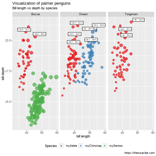<!-- --> ] --- # aspect ratio .pull-left[ ```r tibble(x = 1:10, y = 2*x) %>% ggplot(aes(x = x, y = y)) + geom_line() + coord_fixed() ``` ] .pull-right[ <img src="lec2_files/figure-html/unnamed-chunk-48-1.png" width="90%" /> ] --- # theme `ggplot2` has a lot of [theme](https://ggplot2.tidyverse.org/reference/ggtheme.html). It has even a theme package. .pull-left[ ```r p + theme_bw() ``` * check out `ggthemr` package ] .pull-right[ 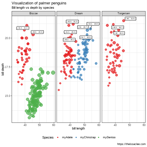<!-- --> ] --- # Box plot ```r ggplot(penguins, aes(y = body_mass_g)) + geom_boxplot() ``` <div class="figure" style="text-align: center"> <img src="lec2_files/figure-html/boxplot1-1.png" alt="One single boxplot" width="30%" /> <p class="caption">One single boxplot</p> </div> --- # Box plot by species ```r ggplot(penguins, aes(x = species, y = body_mass_g)) + geom_boxplot() ``` <div class="figure" style="text-align: center"> <img src="lec2_files/figure-html/boxplot2-1.png" alt="One single boxplot" width="30%" /> <p class="caption">One single boxplot</p> </div> --- # Box plot by species The plot is flipped. Why? ```r ggplot(penguins, aes(x = body_mass_g, y = species)) + geom_boxplot() ``` <img src="lec2_files/figure-html/boxplot3-1.png" width="30%" style="display: block; margin: auto;" /> --- # Box plot by species Add actual values. ```r ggplot(penguins, aes(x = species, y = body_mass_g)) + geom_boxplot(outlier.shape = NA) + geom_jitter(width = 0.2) ``` <img src="lec2_files/figure-html/boxplot4-1.png" width="30%" style="display: block; margin: auto;" /> --- # Box plot with continuous variables You can draw the boxplot using continuous variables ```r ggplot(penguins, aes(x = bill_length_mm, y = body_mass_g)) + geom_boxplot() ``` <img src="lec2_files/figure-html/boxplot5-1.png" width="30%" style="display: block; margin: auto;" /> --- # Box plot with continuous variables You can draw the boxplot using continuous variables ```r ggplot(penguins, aes(x = bill_length_mm, y = body_mass_g)) + geom_boxplot(aes(group = cut_width(bill_length_mm, 5))) ``` <img src="lec2_files/figure-html/boxplot6-1.png" width="30%" style="display: block; margin: auto;" /> --- # Bar chart ```r ggplot(penguins, aes(y = species)) + geom_bar() ``` <div class="figure" style="text-align: center"> <img src="lec2_files/figure-html/barchart-1.png" alt="Bar chart" width="30%" /> <p class="caption">Bar chart</p> </div> --- # Bar chart with `fct_reorder` ```r penguins %>% count(species) %>% ggplot(aes(x = n, y = fct_reorder(species, n))) + geom_col() ``` <div class="figure" style="text-align: center"> <img src="lec2_files/figure-html/barchart2-1.png" alt="Bar chart" width="30%" /> <p class="caption">Bar chart</p> </div> --- # Reference * https://dplyr.tidyverse.org/ * https://ggplot2.tidyverse.org/ * https://ijeamaka-anyene.netlify.app/posts/2020-10-22-workshop-an-introduction-to-ggplot2/ --- class: center, middle # Thanks!